NFL Tracking Data Project
Summary of Project Presented at CASSIS
In Spring 2024, I worked on a project using NFL player tracking data provided by the Kaggle NFL Big Data Bowl. Although I was late to the party and as a result didn’t get to submit anything, I did do some work that got valuable feedback from Professor Greg Matthews along the way.
I was inspired by the submission and subsequent paper
To build on this, I wanted to score players based on yards and points saved rather than momentum decreased. Although it captures a similar notion, I think that putting it in terms of yards and points provides a more intuitive metric by which to evaluate players. To build intuition on the value of both of these metrics, see the GIF below. In week 2 of the 2022 season, the Jaguars thrashed the Colts 24-0. In the fourth quarter, Jonathan Taylor broke off a run for about 25 yards. In the play, number 26 is credited with making the tackle. However, the most valuable defender on the play was clearly number two, who functioned as a speed bump, slowing down Taylor enough for the Jaguars defenders to catch up and make a play. With typical tackle tallying metrics, 2 would not have gotten credit.
With this motivating example, we set off to value a defender’s contribution in terms more fitting. I’ve included the code for this project in a repo on my GitHub.
Valuing Offensive Players
Preparing the Data
The data tracks every player at 30 fps for every play of every game of the first nine weeks of the 2022 NFL season. The player’s position, orientation, and speed are all tracked. Only plays for which the rusher is a running back (RB) are considered, and handoffs are the only play considered. Additionally, plays with a penalty are removed. This still leaves 3.8 million frames to work with. Obviously these frames are not independent, but I believe there is still enough data to produce insights.
Estimating Yards Gained
The approach taken in this project is inspired by other work by Yurko/Nguyen and other CMU contributors, specifically their work on evaluating passing defense, which was presented at NESSIS in 2023 and subsequently published as a paper
We are interested in estimating the yards that an RB will gain. More formally, let $Y$ be a random variable mapping each frame to the yards from the end zone at the end of the play. For each frame, we are interested in the conditional expectation of $Y$, conditional on features of the play relating to the RB position, distances between players, and RB speed. We will use the RFCDE method to estimate
\[\mathbb{E}[Y | \textbf{X}_1] = \sum_{y = 0}^{100} P(Y = y | \textbf{X}_1)y.\]After some tuning, I ended up using only the speed of the RB and the distance from the closest eight defenders to the RB. Additionally, we fit multiple models through a leave-one-week-out crossfitting approach in which each week is left out of the training process, yielding nine models. When estimating the density for a play, we then always work with the model that left out the week in which the play being considered has occurred.
Estimating Instantaneous Value of RB
While the yards gained by an RB is useful, note that not all yards are created equal. For instance, in some cases a defender may decide to give up additional yards in order to increase the likelihood that they can prevent a first down. This is because the defender is really looking to save points rather than yards. Thus, in this section we will extend our model to evaluate defenders by points saved rather than yards saved.
We will be using pre-existing expected points models for this portion of the project, for which there has been much work done. While I won’t go into an extensive review, some important works include Romer’s analysis of the valuation of game states, in which he also discusses fourth down decision making
The XGBoost model developed by Ben Baldwin is publicly available in the nflfastR package, and the one we use here is trained on similar data and features to theirs, with some slight tweaks.
Before diving into the modeling, I want to note that there are shortcomings common to all of these proposed methods. As detailed by Ryan Brill in an outstanding talk at NESSIS 2023, these models do/fail to (1) adjust for team quality, (2) data has selection bias, and (3) effective sample size is much smaller than it would appear. The first issue is difficult to solve because the features offered have complex interactions and nonlinearities. The second issue is a little more sneaky. In the tracking and play-by-play data, good teams end up running more plays, and on those plays scoring more points. Thus, estimates of the expected points models will overestimate the true expected points. Third, frames of the same play and plays on the same drive have the same outcomes in yards and points respectively. Thus, the observations demonstrate high autocorrelation. The diminishing of sample size and biasing of the data exacerbates the first issue of adjusting for team quality, making it more difficult. Ryan explain and demonstrates these issues in much greater detail in his work
With all of that said, I will be sticking with an XGBoost model that is slightly altered from the one made publicly available by nflfastR. For each yard line that the RB could be tackled, we have a game state that would result from that tackle. For instance, if the RB is tackled after gaining three yards on a 1st and 10 at their 25, the resulting game state is a 2nd and 7 at their 28. Additionally, if it is a 4th and 4 and the RB is tackled after gaining only two yards, the other team takes over possession. This gives us a game state including the seconds remaining in the half, yardline, whether the home team has possession, yards to go, the era (see nflfastR, and down. By weighting the probability of the RB being tackled at each of these yardage markers (which we just modeled in the previous section!), we can estimate the expected value of the RB in terms of points rather than yards.
Ranking Defensive Players
A defender’s value comes from their ability to decrease the value of the offensive player. Take the video example from above. The hit on Jonathan Taylor slowed him considerably, allowing defenders to close, decreasing his probability of breaking off a big run, and lowering the expected yards he would gain as well as the expected points of the yard markers at which he was likely to get tackled. Thus, with these models, I will credit defenders for their ability to decrease the value of the RB in terms of yards and points, using the models we just built. This leaves us with the task of attributing credit.
In the momentum-based fractional tackles project from CMU, they consider a defender to have a “contact opportunity” if they are within 1.5 yards of the RB. To choose this number, they examined the distribution of distance from the RB to the nearest defender for the frames with first contact or tackle events. Below is that same plot for the plays and frames that I examined (they used a slightly different subset). The 1.5 yard criteria looks like a perfectly reasonably cutoff for our purposes as well (see below).
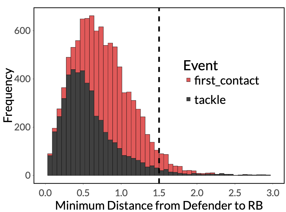
On top of identifying players deserving of credit, there is the question of how to best distribute credit among these players. It can be distributed uniformly (as the CMU project did), but one can also weight defenders by their distance to the RB. The thinking is that closer defenders get more credit and blame for the outcome that defenders on the periphary of the 1.5 yard bubble that can only make arm tackles. At each frame, the inverse distance weights are computed as the proportion of the total distance among defenders that have contact opportunities. Both overall yards/points saved and per-contact opportunity yards/points saved are shown below.
- Overall vs. rate scores
- Tables and outputs
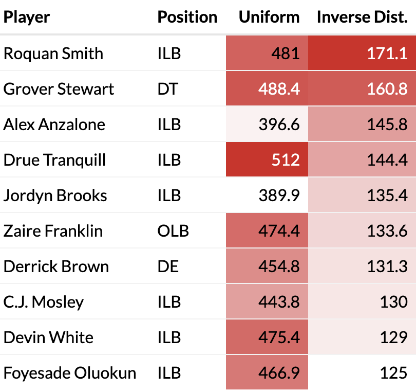
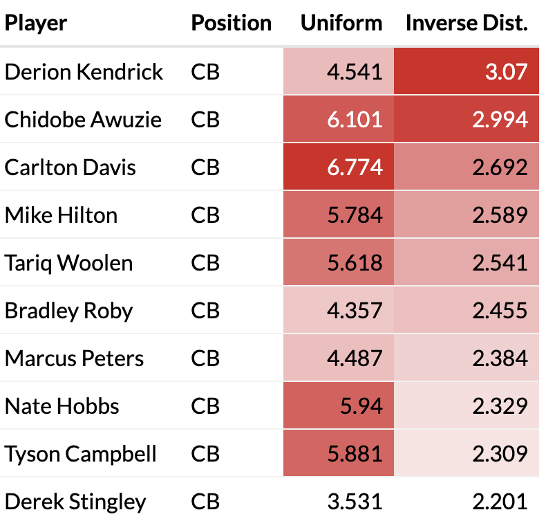
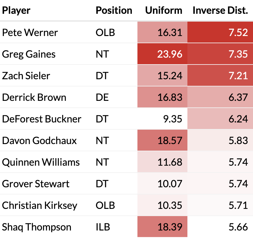
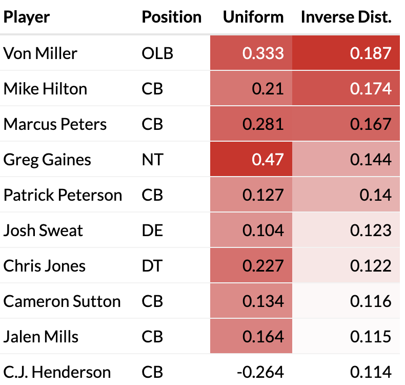
The players that accumulate the greatest totals in yards/points saved are the players that are involved with stopping the run most consistently. Namely, the front seven. The players that save the most yards are the linebackers, who are put into higher-leverage yardage saving opportunities than defensive linemen tend to be. Additionally, the defensive line is primarily responsible to stopping plays like quarterback sneaks and goalline rushes, which gives them high-leverage points saving opportunities. Looking at the top per-opportunity performers, we see mostly cornerbacks, who don’t get tasked with stopping the run as often, but when they have to it is to stop home run plays than a player in the front seven might face. Jonathan Taylor’s run above is one such example.
Wrapping Up
This sort of credits players without worrying about what has happened earlier on the play. We just look at the differences between frames, so a player breaking free is not continuously penalized. This could be interpreted as good or bad. I don’t consider more long range impact where an RB may change direction in anticipation of a defender a few yards down field.